Preface
All of the content here is to be a summary/notes for the multi-armed bandits chapter in the 2nd edition of the book Reinforcement Learning: An Introduction by Sutton and Barto.
What is the MAB problem?
Consider k different slot machines each with different payouts and probabilities of winning. Our goal is to maximize winnings over it without any prior knowledge of the machines.
Think about being in a casino with no one around except you. You’re given 1000 attempts at various slot machines but you have no idea about their dynamics. Naturally you’d want to maximize your profit.
- Let’s say you start off randomly going around trying different machines and note the money you’ve made from each attempt. You do this to gauge the amount of money you can make off of each machine. This is called exploration.
- Now after a while you’ll want to maximize amount of money and use the machine which has best odds based on your observations. This is called exploitation.
Exploration/Exploitation Dilemma
When do you decide to explore more versus exploting already know information?
Determining the balance is broadly based on the estimates we’ve made so far, uncertainties and the amount of turns we have left. There are sophisticated methods which can be applied, but it makes strong assumptions on the problem which are impractical.
In any case we have to determine the value of each machine. In our above scenario a natural estimate is to just average the money earned from each machine as its value.
$$\Large Q_t(a) = \frac {sum\ of\ rewards\ when\ a\ taken\ prior\ to\ t} {number\ of\ times\ a\ taken\ prior\ to\ t} = \frac {\sum_{t=1}^{t-1} R_i.1_{A_i=a}} {\sum_{t=1}^{t-1}1_{A_i=a}}$$
1 is a function which equates to value 1 if its predicate is satisfied . In our case its if action is equal to a.
This approach is called sample-average, and converges to the true value of the action given large amount of samples.
We can perform the exploitation part of our strategy by a greedy selection of actions based on the sample-average value we just discussed.
$$ \Large A_t = argmax_aQ_t(a) $$
By following this equation for action selection, we maximize immediate profit. But in order to explore other machines once in a while, we change this step slightly. We introduce a small probability $\Large \epsilon$ where select an action randomly from all actions independent of the current greedy action. This is known as $\large \epsilon\ greedy$ action selection rule.
Exercise 2.1
In ε-greedy action selection, for the case of two actions and ε = 0.5, what is the probability that the greedy action is selected?
Here since $\large \epsilon$ is 0.5, chance of selecting the greedy action is 1 - $\large \epsilon$ = 0.5
Exercise 2.2
Timestamp Action Reward 1 1 1 2 2 1 3 2 2 4 2 2 5 3 0
Consider the above bandit actions with 4 actions using ε-greedy selection. Where did the exploratory action take place definitely? Where did it possibly occur?
Here in timestep 2, the exploratory action occurred since it has observed that action 1 yielded reward 1 which is greater than 0 for the other actions. It definitely occured at timestep 5 since the reward is 0 and it wasn’t the greedy choice of action 2.
Epsilon Greedy vs Greedy
Epsilon greedy isn’t always the clear choice for an action selection strategy. It’s based upon the variance in the rewards. The larger the variance, the better epsilon greedy fares. In case the variance is zero, then the greedy selection fares better after exploring each action once.
The other section where epsilon greedy fares better is in non-stationary rewards i.e rewards that change over time. Even in this case, the algorithm can keep up.
Efficient way of computing sample-averages
As we have seen, computing the sample average involves a summation over timesteps. Recalculating it each time for an update is inefficient.
There is an incremental version of the same formula used earlier which requires constant memory.
$$ \Large Q_{n+1} = Q_n + \frac{1}{n} \Bigl[R_n - Q_n\Bigr] $$
The equation above can be generalized to an update rule of the form
$$\large NewEstimate \leftarrow OldEstimate + StepSize\Bigl[Target - OldEstimate\Bigr]$$
Nonstationary Rewards
We mentioned nonstationary rewards i.e reward probabilities that change over time. In these situations it makes more sense to weigh the recent rewards more than long term rewards. One way to do this is to keep a constant step-size $\large \alpha$ instead of $\large 1/n$
$$\Large Q_{n+1} = Q_n + \alpha \Bigl[R_n - Q_n\Bigr]$$
This is known as exponential recency-weighted average as the rewards from the past are considered in exponentially decreasing weightage.
Initial values for $Q_n$
In a sense $Q_n(a)$ depends on what initial values we set at the first timestep for the actions. Even if we set all of them to zero, it is still influencing what the future values become. It’s effect reduces as we increase the number of timesteps and is usually not a problem.
But we can take advantage of this bias and use it to supply information to the function with estimates of the rewards. This allows us to design a fully greedy system provided we set the rewards to a “large” value to being with. It causes the system to try an action first and once it sees that the rewards was lower than expected, it will explore another action. This way it is in a constant state of exploring until it converges to the true reward values.
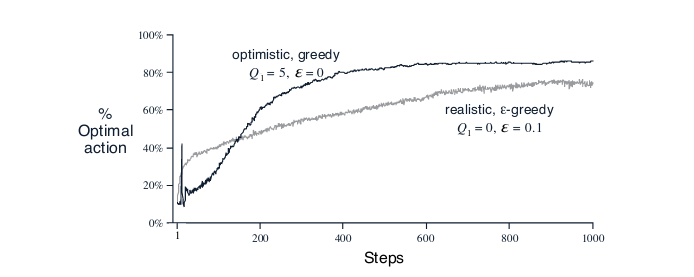
Greedy vs $\large\epsilon$-Greedy with large initial values.
From Reinforcement Learning: An Introduction, Page 27 by Sutton and Barto
We can see that the greedy version converges faster than the $\large\epsilon$-greedy even though it is just acting greedily. The constant updates to rewards causes it to explore more.
This technique works well for stationary problems (environment doesn’t change its rewards over time), but for non-stationary it is only a temporary boost to exploration.
Upper-Confidence-Bound Action Selection
$\large\epsilon$-greedy still has a problem we haven’t considered. It picks the exploratory action at random, paying no heed to whether it has been explored already or not.
Instead we would pick actions to explore based on how uncertain we are of their values i.e based how often we have already explored them. One way of doing this is via this form for action selection
$$\large A_t = argmax_a \Bigl[Q_t(a) + c\sqrt{\frac{\ln(t)}{N_t(a)}}\Bigr]$$
Instead of exploring randomly, we pick the action based upon two parts
- The current reward value $Q_t(a)$
- The square root term $c\sqrt{\frac{\ln(t)}{N_t(a)}}$
The exploration aspect comes from the square-root term where $\ln(t)$ is the natural logarithm of the number of time steps taken till now, denominator $N_t(a)$ the number of times the action has been explored and $c$ controls the degree of exploration. This way less-explored actions will be selected more often. If $N_t(a) = 0$ then it will be chosen over other actions.
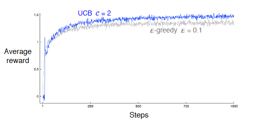
UCB vs $\large\epsilon$-Greedy.
From Reinforcement Learning: An Introduction, Page 28 by Sutton and Barto.
Gradient Bandit Algorithms
This is a different approach to action selection where instead of selecting an action based on maximizing reward values, we instead just define a preference for what action we’d like to perform. Its sort of like sorting all the actions based on preference and for each timestep choose the highest one. The preference is given by a function $H_t(a)$ and action selection is made via a softmax function:
$$Probability\ of\ choosing\ (A_t = a)\ from\ k\ actions= \frac{e^{H_t(a)}}{\sum\limits_{b=1}^{k} e^{H_t(b)}} = \pi_t(a)$$
The initial values for $H_t(a)$ is 0 for all actions $a$.
The update rule for the preferences is given by the following equations
- $H_{t+1}(A_t) = H_t(A_t) + \alpha(R_t - \bar{R}_t)(1 - \pi_t(A_t))$ for the current action taken $A_t$
- $H_{t+1}(a) = H_t(a) - \alpha(R_t - \bar{R}_t)\pi_t(a)$ for all actions $a \neq A_t$
Here $\alpha$ is the step-size parameter and $\bar{R}_t$ is the average of the rewards computed incrementally by the formula from earlier. Note that this average reward is independent of the action chosen.
Also we can substitute $\bar{R}_t$ with any constant or term that does not depend on the selected action and the algorithm will still converge to optimal values.
Associative Search (Contextual Bandits)
Consider our casino problem again. First there were just a bunch of slot machines and our goal was to find the best machine as soon as possible and maximize our profit.
Let’s add another dimension to the problem. Let’s say the colors of all the machines change after every action you take. On every color change, the reward functions associated with the slot machines change accordingly. This way instead of one k-bandit problem, you have multiple k-bandit problems to solve. We’ll need different collections of $Q_t(a)$ ( or $H_t(a)$) for each colored k-bandit problem.
Now we have to search for the solution for each associated colored k-bandit problem. This association will allow us to figure out what action to take under the context of the color of the slot machines. Deciding on an action based on the context is known as a policy. If the actions we take in each step affects the next type of color, then we have a full-reinforcement problem at hand.
Other approaches
There are a couple more ways to solve for multi-armed bandits; Posterior Sampling and Gittins indices, which I still haven’t been able to grasp fully and might deserve a blog post of their own.
Conclusion
So we’ve seen a multitude of ways to solve for multi-armed bandit problems both stationary and non-stationary. But these are still just one instance of the full reinforcement problem with a fixed context. We’ll still need to generalize our solution to Contextual Bandits problem with larger space of contexts (color, size, brand and so on).